

Monte Carlo simulations are a mathematical technique used across a diverse range of industries and fields to model difficult-to-predict scenarios and outcomes. Despite their name, you don’t have to be a gambler to appreciate their value—in fact, Monte Carlo simulations were designed to take the gamble out of strategic decision-making processes by forecasting a wide range of potential outcomes of uncertain or unforeseen events.
Spreadsheets are well-suited to this kind of data modeling, and learning how to run Monte Carlo simulations in Microsoft Excel or similar software can add a powerful predictive tool to your decision-making toolset. Follow along as I create a Monte Carlo simulation using a normal distribution to generate random variables to learn how to use this valuable technique in your own work.
- What is a Monte Carlo Simulation?
- Step 1: Set Up Your Monte Carlo Simulation
- Step 2: Create Rows for Your Trials or Iterations
- Step 3: Generate Your Random Value Variables
- Step 4: Verify Your Values
- Step 5: Visualize Your Monte Carlo Simulation Results
- Using Other Monte Carlo Simulation Distribution Types in Excel
- Limitations of Monte Carlo Simulations in Excel
- Excel Add-Ins for Working with Data
- Frequently Asked Questions (FAQs)
- The Bottom Line: Running Monte Carlo Simulations in Excel
What is a Monte Carlo Simulation?
In simple terms, a Monte Carlo Simulation is a virtual representation of any statistical procedure that uses randomly generated numbers to solve a problem—more specifically, it generally refers to generating an array of results known as a distribution for any statistical problem that includes a wide range of inputs sampled over and over again.
Imagine yourself throwing dice. If you throw them hundreds of thousands or even millions of times, you begin to understand the odds of certain combinations coming up. Monte Carlo Simulations replicate this idea, letting us perform the same kind of statistical analysis quickly and efficiently. By varying the inputs, you can model a wide range of possible outcomes and compare them to help you make decisions in the real world, making this a popular and powerful predictive tool for businesses.
Step 1: Set Up Your Monte Carlo Simulation
Let’s say you’re creating a human resources report about salary levels at other similar companies in your industry. To build this report, you need a fictional but accurate representation of annual salaries per employee at a competing company.
You have data that suggests the average (mean) annual salary is $40,000, and the standard deviation is $10,000. You want to generate a random salary value based on a normal distribution with the specified mean and standard deviation—each time you recalculate the formula, it should generate a new random salary that follows the given distribution.
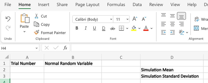
The first step is to set up the simulation in a blank Microsoft Excel sheet as follows:
- Create two columns labeled “Trial Number” and “Normal Random Variable.”
- Create two fields with corresponding labels for “Simulation Mean” and “Simulation Standard Deviation.”
The mean—often referred to as the arithmetic mean or average—is a statistical measure of central tendency that represents the sum of a set of values divided by the total number of observations in that set.
Standard deviation and average/mean calculations are indispensable for ensuring your simulation conforms to expectations.
Standard Deviation
Standard deviation measures the amount of variation or dispersion in a set of values by quantifying the extent to which the individual values in a dataset deviate from the mean.
- A low standard deviation indicates that the values tend to be close to the mean.
- A high standard deviation suggests that the values are spread out over a wider range.
Standard deviation is calculated by taking the square root of the variance—the average of the squared differences between each data point and the mean. When used together, the average/mean and standard deviation provide a more complete picture of the characteristics of a dataset. This allows you to assess the spread of data points and make informed conclusions about the variability and reliability of the dataset under analysis.
Normal/Gaussian Distribution
Monte Carlo simulations generate a series of random observations based on a specific type of statistical distribution. These distributions can be represented as probability curves that determine the likelihood of a particular outcome.
The Monte Carlo simulation I’m creating for this example uses a normal, or Gaussian, distribution—as a result, you can expect about 68 percent of the data to fall within one standard deviation of the mean, 95 percent within two standard deviations, and approximately 99.7 percent within three standard deviations.
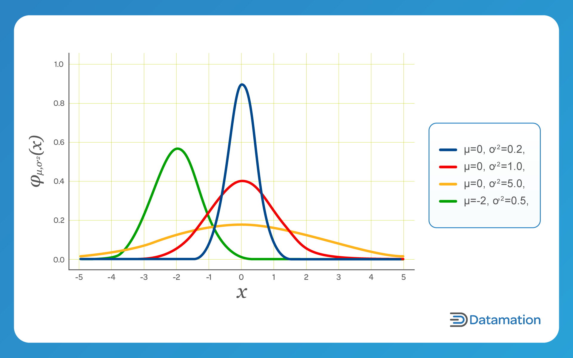
The normal or Gaussian distribution is perhaps best known for its visual representation as the standard bell-shaped curve; when plotted, this function is characterized by an even distribution on each side, with tails that stretch to infinity on the X-axis.
In normal distributions, the median and mean values are the same—this leaves zero skew and a symmetrical graph. Normal distributions are appropriate for continuous data that has an equal likelihood of being above or below the mean, and are commonly used for measuring continuous data that hovers around a mean value. For example, instructors typically grade their students’ test scores on a normal distribution curve as a way to ensure fairness.
Step 2: Create Rows for Your Trials or Iterations
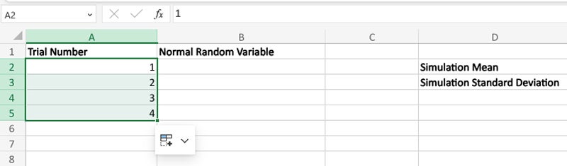
In this example, let’s simulate 100 trials or iterations for a normal random variable with a mean of 40,000 and a standard deviation of 10,000. Here’s how to set that up in the Excel sheet:
- In the “Trial Number” column, insert the first two sequential values (1 and 2) manually in the first two rows below the header.
- Highlight the two values—the draggable green edge will appear on the bottom right of the selection.
- Drag the green edge down the column to create 100 sequential row values in the “Trial Number” column.
Step 3: Generate Your Random Value Variables
Monte Carlo simulations in Excel rely on two functions in particular: RAND() and NORM.INV. The first, RAND(), introduces variability to simulate randomness by using a built-in formula to generate a random numeric decimal value between 0 and 1. The second, NORM.INV, returns the inverse of the normal cumulative distribution for the specified mean and standard deviation—in this example, 40,000 and 10,000 respectively.
To generate these values:
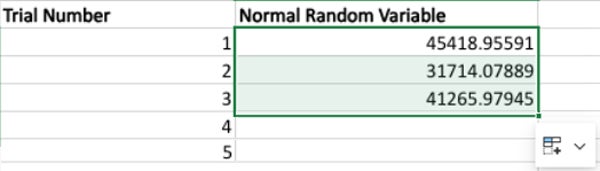
- Insert the following formula into the first field of your “Normal Random Variable” column:
=NORM.INV(RAND(),40000,10000)
- Select the value and drag the green edge down the column until you have 100 normal random variables for row values.
Step 4: Verify Your Values
If you take a cursory glance at your resulting values, you’ll notice that they look fairly normal in terms of the distribution—as they should. We can verify this by calculating the mean/average and standard deviation for the entire generated dataset in your Monte Carlo Simulation:
- Insert the following formula into the field next to your “Simulation Mean” label to get the mean/average:
=AVERAGE(B2:B101)
Be sure to replace “B2:B101” with the actual data range in your spreadsheet.
- Insert the following formula into the field next to your “Standard Deviation” label to get the standard deviation for the data set:
=STDEV(B2:B101)
Again, be sure to replace “B2:B101” with the actual data range in your spreadsheet.
WIth these steps completed, your Monte Carlo Simulation results should resemble my outputs in the illustration below.
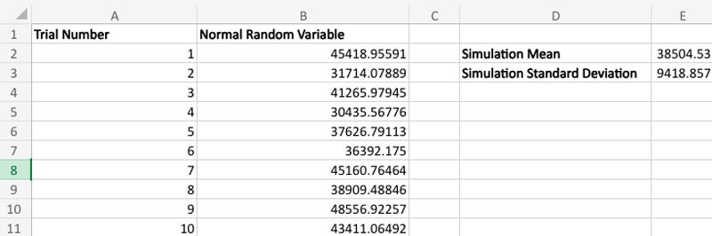
In comparing the hard-coded, specified average/mean and standard deviation values with the average/mean and standard deviation values generated from the simulated dataset, you’ll see that the values seem to be in line with expectations.
| Average (mean) | Standard Deviation | |
|---|---|---|
| Specified | 40,000 | 10,000 |
| Simulation | 38504.53 | 9418.857 |
Step 5: Visualize Your Monte Carlo Simulation Results
Since we used the NORM.INV function to create your normal random variable values, the plot should resemble a standard bell-curve distribution. You can verify this in Excel by plotting out your results in a histogram;
- To verify that your results conform to the expected normal distribution curvature, select all the values in the “Normal Random Variable” column.
- Next, select the “Insert” menu, and click the small arrow to expand the ribbon and show all available chart options.
- Select “All Charts,” and choose Histogram from the list.
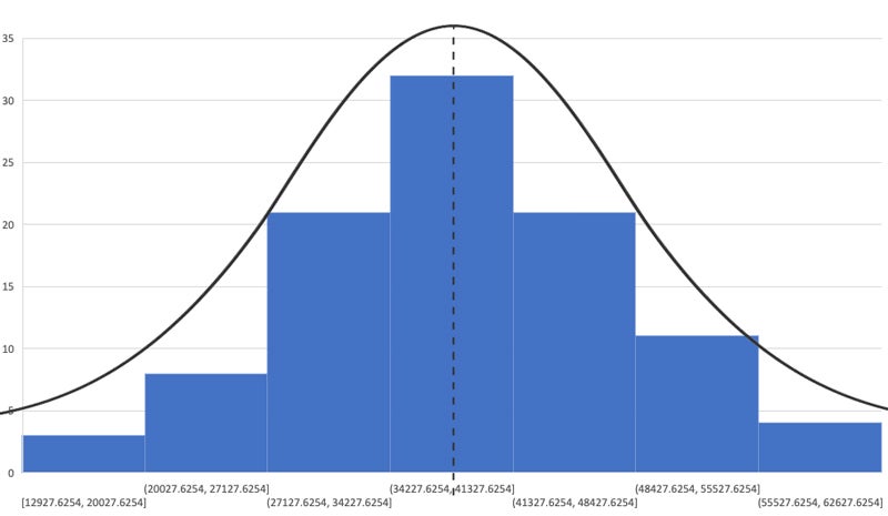
- The resulting histogram visually represents the distribution of outcomes, grouped into bins, as in the following image.
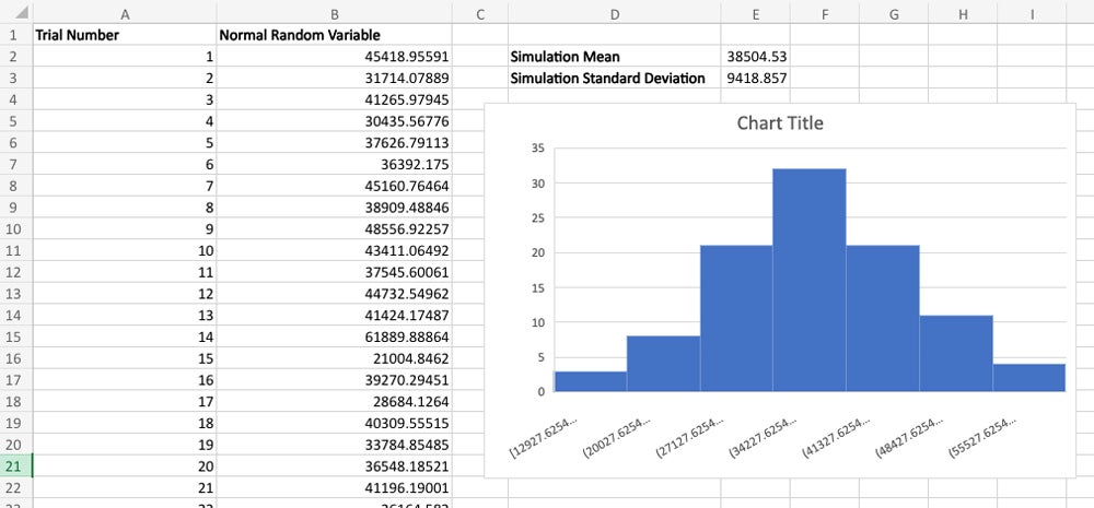
As you can see, your Monte Carlo simulation conforms to a standard distribution—you can trace the lines contours of a bell-shaped curve on the outer edges of the histogram.
Remember, our goal was to create a fictional representation of annual salaries at a company similar to your own in order to generate an HR report about salary levels at competing businesses, and your data suggested an average (mean) annual salary of $40,000 with a standard deviation of $10,000.
Using the results of our Monte Carlo simulation, you have a scientifically-derived sample dataset of hypothetical competitor salaries to compare against your own.
Using Other Monte Carlo Simulation Distribution Types in Excel
Along with normal/Gaussian distributions, Excel provides a number of statistical distribution types to use in Monte Carlo simulations.You can find them under the Formulas menu by selecting “More Functions” and then “Statistical.” There are a few that I find more useful than others, as they represent the more common distribution types.
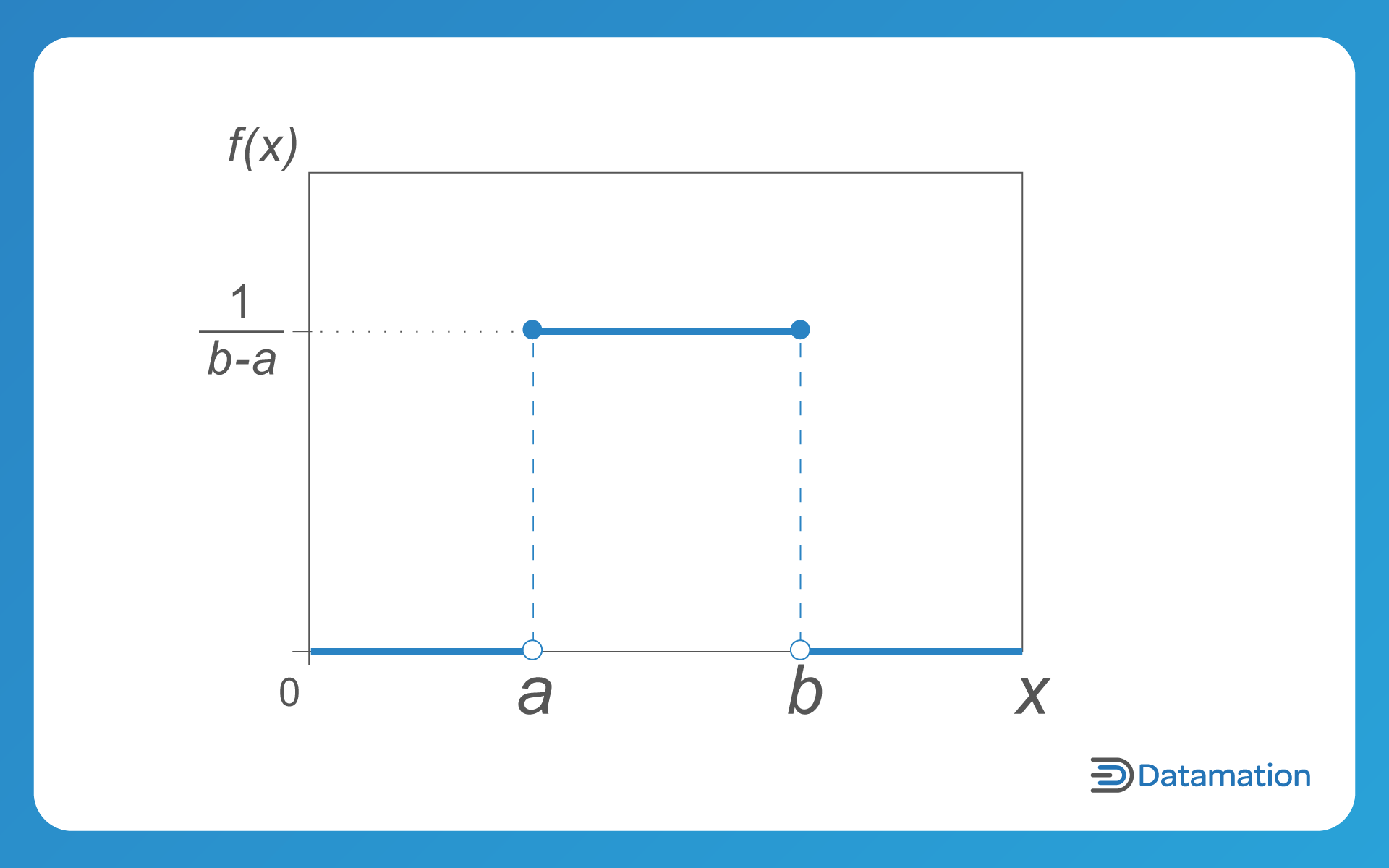
Uniform Distribution
In a uniform distribution, an equal likelihood exists between the minimum and maximum values. Visually, a uniform distribution looks like a rectangle when plotted out on a graph. Uniform distributions are often used to generate random numbers and in other scenarios that involve events that are equally likely to occur.
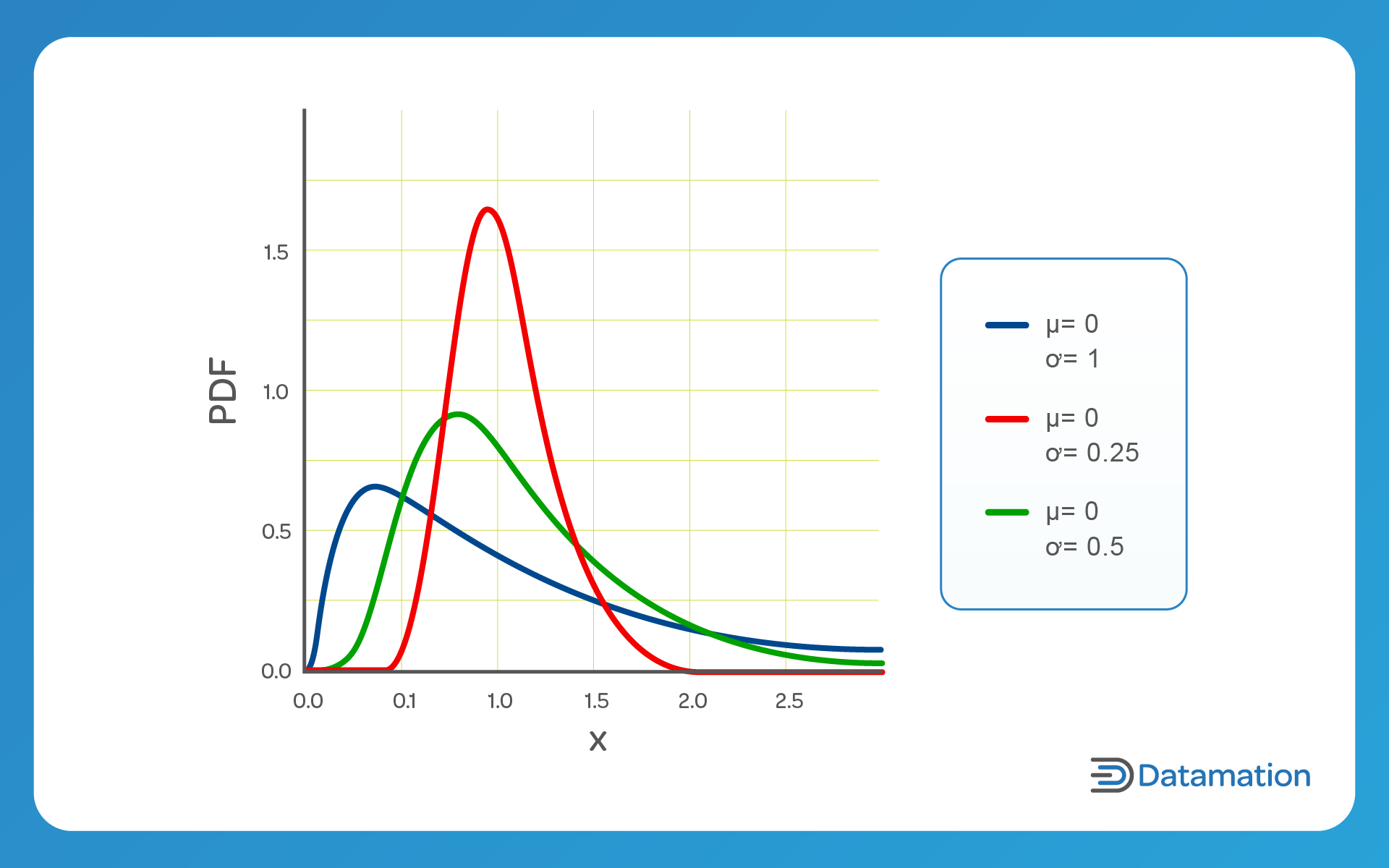
Log-Normal Distribution
As its name implies, a log-normal distribution has a normally distributed logarithm with the mean and standard deviation. Log-normal distributions skew to the right and are ideal for modeling rate descriptions—for example, time to repair, equipment failure rates, and income distributions.
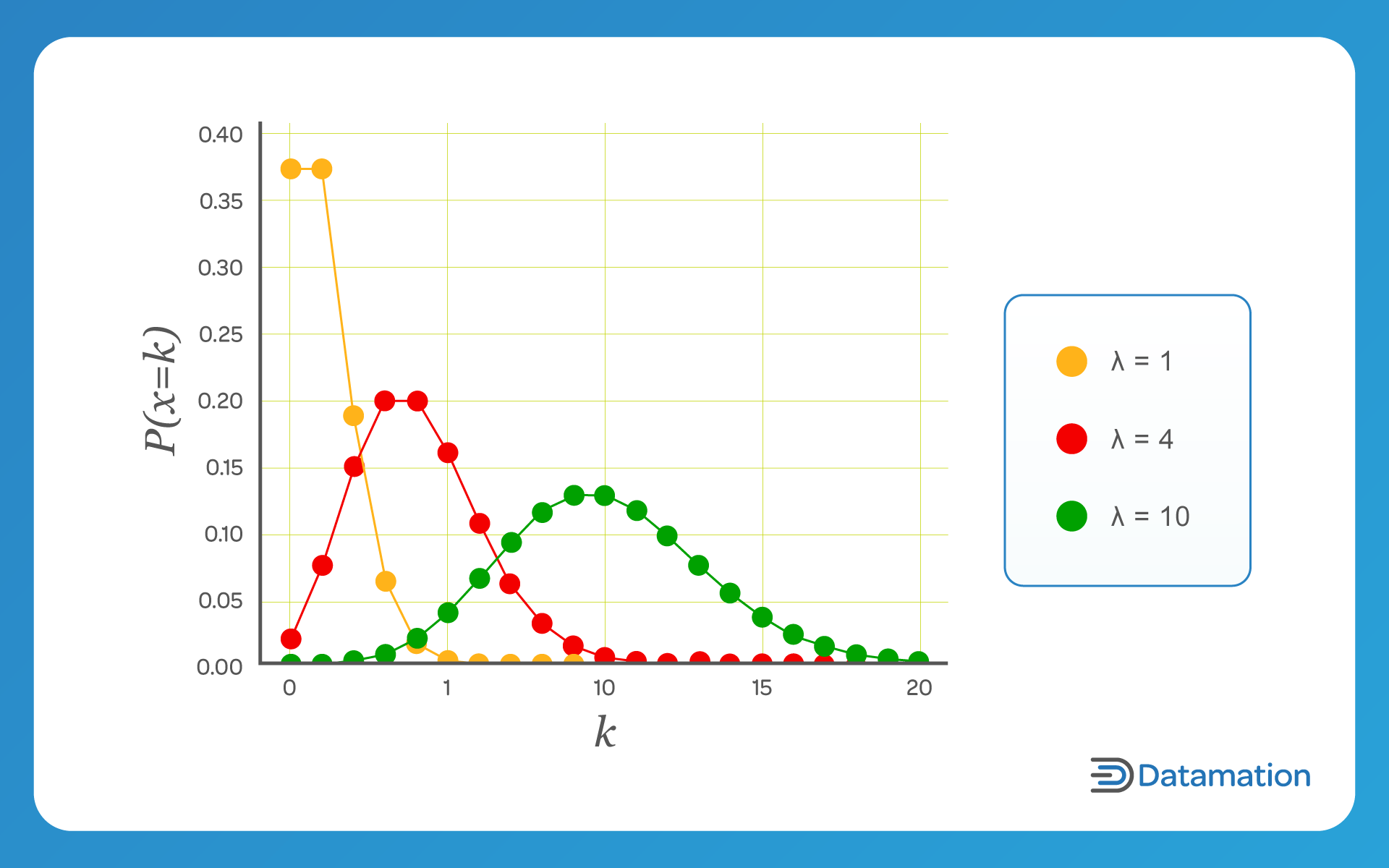
Poisson Distribution
Poisson distributions are ideal for addressing large distributions near the start that quickly dissipate to a long tail on one side. They’re best for predicting the number of events that transpire within a given timeframe—for example, customer purchases per quarter or transactions per day.
Limitations of Monte Carlo Simulations in Excel
Excel can be a useful tool for many Monte Carlo simulations, but the software’s limitations as a desktop or Software as a Service (SaaS) application are worth keeping in mind.
Random Number Generation
Excel’s built-in random number generator uses a pseudorandom number generator, and the quality of randomness may be a concern in certain use cases. Advanced simulations might require more sophisticated random number generation techniques.
Limited Flexibility for Complex Models
Excel may not be suitable for highly complex models that involve intricate interdependencies, non-linear relationships, or dynamic systems. I suggest using specialized simulation or statistical software or programming languages in these cases.
Limited Support for Advanced Techniques
Some advanced Monte Carlo simulation techniques such as adaptive sampling or advanced variance reduction methods are difficult to implement in Excel without resorting to complex workarounds.
Lack of Parallel Processing
Unlike a cloud-based data warehouse or statistical package, Excel is incapable of parallel processing and horizontal scaling. This limits its performance capabilities when carrying out simulations, as it lacks the parallelization mechanisms to speed up computations.
Excel Add-Ins for Working with Data
Data simulation—generating synthetic data to closely mimic the properties and characteristics of real-world data—can offer data scientists, engineers, and commercial enterprises access to training data at a fraction of the cost of real world data and open doors to all kinds of predictive modeling, risk assessment, and other benefits.
Monte Carlo simulations are just one example of what’s possible—and while Excel’s wide range of statistical functions is sufficient for them in many cases, it lacks some of the more advanced statistical analysis tools required for in-depth analysis of simulation results. For this, I recommend that you install one of the many third-party and Microsoft-provided statistics add-ons directly from within Excel.
Even with add-ins, however, desktop spreadsheet applications are not designed for heavy computational tasks. As the number of simulations or the complexity of the model increases, computation times can quickly overcome your system. For large-scale simulations, specialized statistics software packages or programming languages may be more efficient for advanced modeling purposes.
Frequently Asked Questions (FAQs)
How accurate are Monte Carlo simulations?
Monte Carlo simulations estimate numerical results through random sampling, so the accuracy of the Monte Carlo simulation method increases with your sample size. That said, the accuracy level is also influenced by other factors such as the quality of the random number generator—for example, Excel’s random number generator is limited in this regard.
How many Monte Carlo simulations is enough?
The ideal sample size for your Monte Carlo simulation depends on various factors, including the desired level of precision and the characteristics of the modeled system/scenario. But you can use more advanced statistical tools to determine your ideal sample size. For example, running a sensitivity analysis will let you determine how changes in sample size impact the stability/reliability of your simulation; this involves running the simulation with different sample sizes and observing the variation in outcomes.
Do Monte Carlo simulations assume a normal distribution?
Generally speaking, all simulations will assume a normal distribution if your sample size is large enough; however, depending on the specific context/nature of the simulated data, one of the other distribution types may be more appropriate for your use case. Running a sensitivity analysis will allow you to compare how different data distributions affect your outcome.
Can I run a Monte Carlo simulation using software other than Excel?
Yes, you can use comparable spreadsheet programs like Google Sheets or Zoho Sheets to run a Monte Carlo simulation. Advanced statistical software packages like IBM SPSS and SAS offer more power and options when running Monte Carlo simulations, at the cost of a steep learning curve.
The Bottom Line: Running Monte Carlo Simulations in Excel
Monte Carlo simulations are easy-to-use, powerful mechanisms for enterprise decision-making, risk assessment, and forecasting. Despite some limitations, Excel and similar spreadsheet tools remain competent options for carrying out rudimentary Monte Carlo simulations and should prove an indispensable statistical instrument in your analytical toolkit. For more sophisticated applications, I recommend that you consider specialized simulation software packages or programming languages like Python, R, or MATLAB.
If you’re interested in Monte Carlo simulations, learn more about how data modeling differs from data architecture or read our comprehensive guide to logical and physical data models.