As I showed in my first Excel functions article, the serious meat in any spreadsheet is the formulas and functions that perform the calculations. Excel offers functions that you can use to make the process of computing the results simpler for many standard calculations. In this article I’ll show you some useful examples; I’ll tell you how to find functions to perform specific tasks and what to consider when building your own formulas.

Practical Formulas

Probably the first function you’ll have learned to use is =SUM, which calculates the sum of a range of numbers. This saves you from having to build simple additions one cell at a time. However this function will fail spectacularly if you have a filtered list.

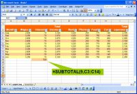
The SUBTOTAL function is required when totaling only visible values in a filtered list. (Click for larger image).

If you filter a list to show only a small range of numbers and use =SUM to total the visible numbers –you’ll be disappointed as the function sums all values in the selected range – visible and not. Instead, when you total a filtered list you must use the SUBTOTAL function and, in fact, if you select the AutoSum button to calculate the sum automatically Excel will apply the SUBTOTAL function where the area to sum is a filtered list.

Once you know the limitations you can write your own SUBTOTAL function – it’s essentially the same as the SUM function but with an extra argument: =SUBTOTAL(9,A2:A10) – the number nine is the trigger that makes the SUBTOTAL function sum only the visible numbers in the filtered range A2:A10.

Working with Days

When planning projects and calculating timeframes, you often need to know the number of workdays between two dates. The NETWORKDAYS function can do this ‑‑ it calculates the number of days between two dates ignoring Saturdays, Sundays and any holidays that you specify. You’ll find the function in the Excel Analysis Toolpak. To check if the Toolpak is installed, choose Tools > Add-ins and then select the Analysis Toolpak checkbox.

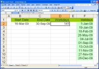
Use the Analysis Toolpak’s NETWORKDAYS function to calculate the workdays between two dates. (Click for larger image).

To use the NETWORKDAYS function, enter the holiday days as a series of dates. Select the cells containing the dates and name them by choosing Insert > Name > Define; type in the holidays and press OK. To calculate the NETWORKDAYS, type the start and end dates in cells A1 and A2. The formula =NETWORKDAYS (A1,A2,holidays) will return the number of workdays between the two dates excluding weekends and the dates in the range you’ve named holidays.

Two other useful date functions are =NOW() and =TODAY(). The function =NOW inserts the current date and time into the cell and the =TODAY function enters the current date. You may need to format the cells to a date or time format using Format > Cell > Number Format for the date and time data to show correctly.

Referring to a Cell

To refer to the contents of one cell in another cell, type the cell reference with an = symbol. So, to refer to the contents of cell C2 in another cell, type =C2. If the value in cell C2 changes in the future, this cell’s value will change, too. You can also refer to a cell on another worksheet by including the sheet name – for example, to refer to the contents of C2 in Sheet 3 of the workbook use =Sheet3!C2.

Multiply and Add

Some calculations, such as computing the value of your inventory, require a two-step process of multiplying values and then adding the results. You can reduce the work by using the SUMPRODUCT function.

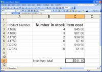
Calculate the total value of your inventory using the SUMPRODUCT function. (Click for larger image).

This function takes two ranges and multiplies each element in the first range by each matching element in the second range, and then it totals the result. For example, if your inventory worksheet includes numbers of each item in column B (rows 2 – 25) and the corresponding cost value in column C, you can calculate the overall value with this function:

=SUMPRODUCT(B2:B25,C2:C25)

Finding a Function

If you are unsure which function to use for a particular task, you can get assistance from Excel itself. Click in the cell where the function should appear, choose Insert > Function and type a brief description of what you want to do.

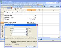
Alternatively, select the category of function, for example Financial Functions and look for a function to perform the required task. Select the function to see a description of what it does and the data it requires. When you click OK the Function Arguments dialog appears, and you can select each item in turn to build your formula. Arguments in bold type are required and those in regular type are optional. Check the Function Arguments dialog for any specific information about the data the function requires.

Using Insert > Function gives you additional tools for locating and using Excel functions. (Click for larger image).

If you have already started entering a function and you decide you need more help, press Ctrl + A to display the function arguments dialog. This gives you step-by-step assistance in completing the function.

Things to Keep in Mind

When a particular calculation has no built-in function, you can build your own Excel formula. When doing so, take care that you don’t fall foul of the order in which Excel makes calculations. For example, Excel calculates =2+3*4 as 14 not 20 because it performs calculations in a particular sequence called the order of precedence.

Thus Excel performs multiplication and division before addition and subtraction so the 3*4 part of the formula is calculated before adding the result to the number 2. If the answer should be 20, then you must put brackets around the 2+3 part of the calculation to force it to be performed before the multiplication ‑‑ brackets take precedence over multiplication and division. This formula will give a result of 20: =(2+3)*4

An instance where you may encounter the need to put calculations in brackets is when you are calculating tax on a price less a discount. If you’re selling an item for $100 with a $10 discount and tax is 7 percent of the total, then you will use =(100-10)*7% to calculate the tax ‑‑ without the brackets the result would be incorrect.

If you are using a function that you are unfamiliar with, always test it first with data for which you know the answer already so you can check to ensure it is working correctly.

Helen Bradley is a respected international journalist writing regularly for small business and computer publications in the USA, Canada, South Africa, UK and Australia. You can learn more about her at her Web site, HelenBradley.com

This article was first published on SmallBusinessComputing.com.